9.1 Logistic Regression

If we are analyzing a binary outcome, we can use logistic regression. Logistic regression uses the linear model framework, but makes different assumptions about the distribution of the outcome. So we can look for associations between binary outcome variables and multiple explanatory variables.

ggplot(cats, aes(x = roamer, y = wander_dist)) + 
  geom_boxplot(width = 0.5)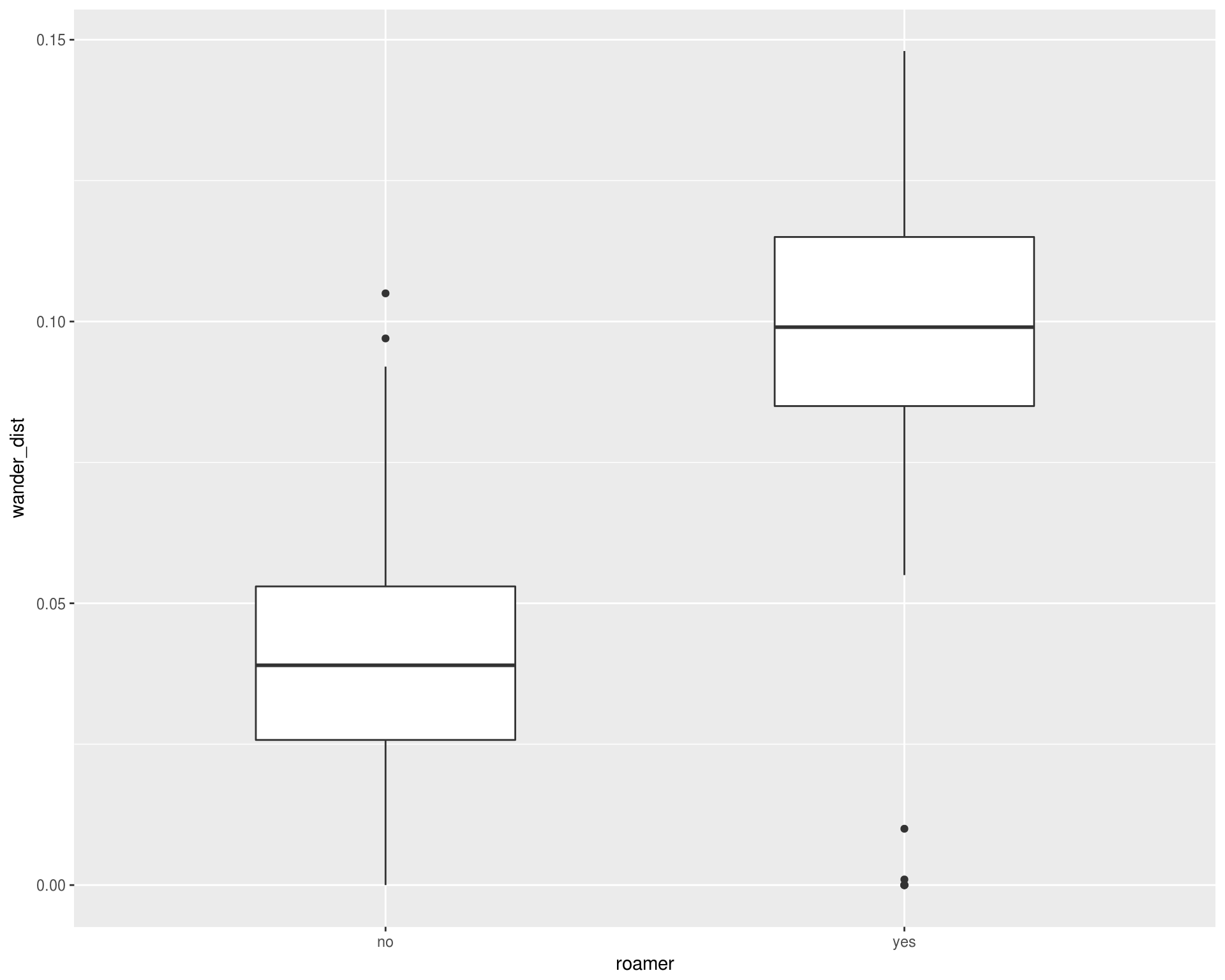

---

For logistic regression, we use the glm function. It takes formula and data arguments like the lm function, but we also need to specify a family. For logistic, we pass binomial as the family, which tells the glm function that we have a binary outcome, and we want to use the logit link function.

roamer_fit <- glm(formula = roamer ~ wander_dist, data = cats, family = binomial )

---

We can use the summary function to extract important information from the object that glm returns, just like with the lm function

glm_summary <- summary(roamer_fit)
glm_summary

9.1 Challenge

roamer_fit <- glm(formula = roamer ~ wander_dist + weight, data = cats, family = binomial )
summary(roamer_fit)

---

We can look at the effects of multiple covariates on our binary outcome with logistic regression, just like with linear regression. We just add as many variable names as we’d like to the right side of the formula argument, separated by + symbols.

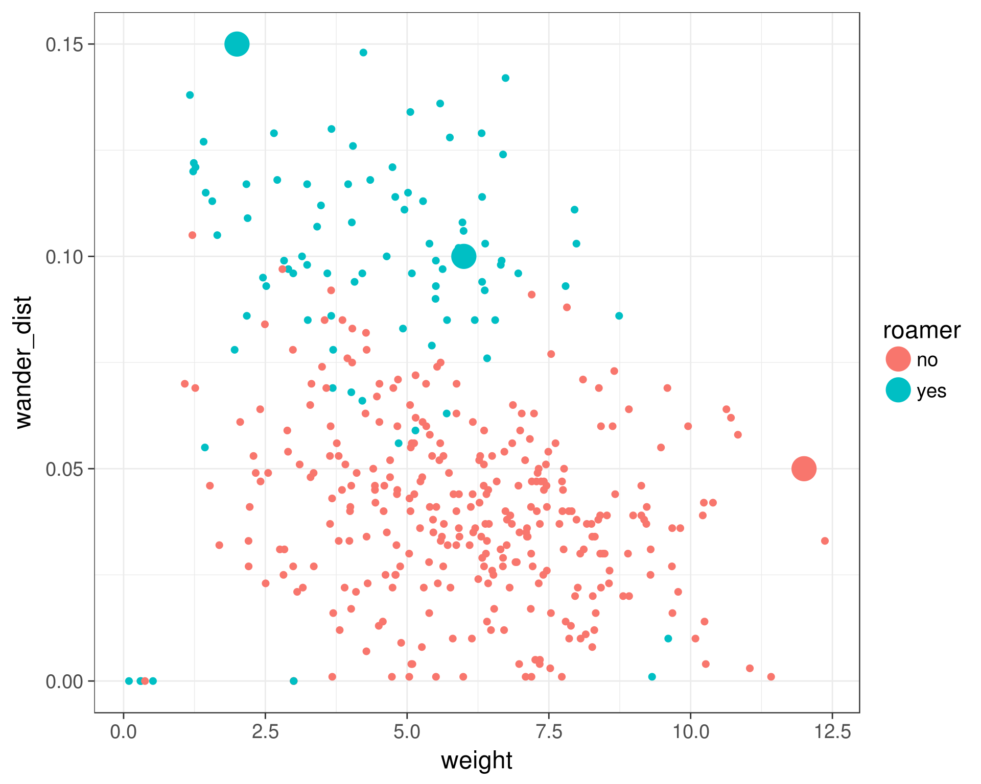
ggplot(cats, aes(x = weight, y = wander_dist, color = roamer)) + 
  geom_point(size = 2) +
  geom_smooth(method = 'lm', se = FALSE, size = 3) +
  theme_bw(base_size = 18)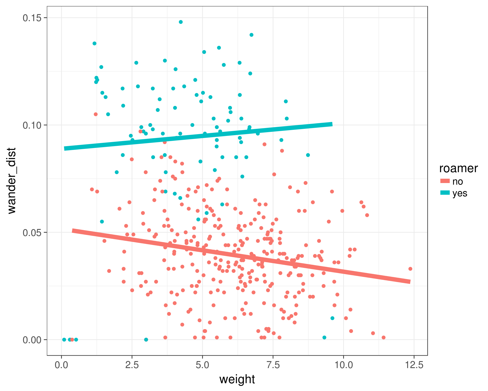

# cats$roamer <- relevel(cats$roamer, ref = 'yes')
roamer_fit <- glm(formula = roamer ~ wander_dist + weight, data = cats, family = binomial )
glm_summary <- summary(roamer_fit)
glm_summary

names(glm_summary)
glm_summary$coefficients
glm_summary$null.deviance
glm_summary$deviance
glm_summary$aic

---

We can also use the model objects to predict on unobserved values. We just need to pass a data frame with all of the terms used in the original model to the predict function. The predict function will return values in a few different ways. The default value of the type argument is “link” and will return things on the same scale as the linear predictors. This is often not what we want. If we pass “response” to the type argument, we’ll get predicted values on the same scale as the response. In the logistic case, this is the predicted probability.

new_cats <- data.frame(wander_dist = c(0.15, 0.10, 0.05),
                       weight = c(2, 6, 12))
new_cats

predicted_logit <- predict(object = roamer_fit, newdata = new_cats)
predicted_logit

predicted_probs <- predict(object = roamer_fit, newdata = new_cats, type = 'response')
predicted_probs

---

We can then predict whether each cat is a roamer or not based on the predicted probabilty from our model. We need to assign a cut-off probability.

new_cats$predicted_prob <- predicted_probs
new_cats <- new_cats %>% mutate(roamer = ifelse(predicted_prob > 0.5, 'yes', 'no'))

ggplot(cats, aes(x = weight, y = wander_dist, color = roamer, group = roamer)) + 
  geom_point(size = 2) +
  geom_point(data = new_cats, aes(x = weight, y = wander_dist, color = roamer), size = 8) +
  theme_bw(base_size = 18)

---