Lesson 9 Common Statistical Techniques in R

---

9 Learning Objectives

• To become familiar with common statistical functions available in R
• Linear Regression
• Logistic Regression
• K-Means Clustering

---

9.0.1 Simple Linear Regression

Linear regression is one of the most commonly used methods in all of statistics. It is used for a large variety of applications and offers highly interpretable results. It was the first regression method discovered and belongs to one of the most important families of models, generalized linear models.

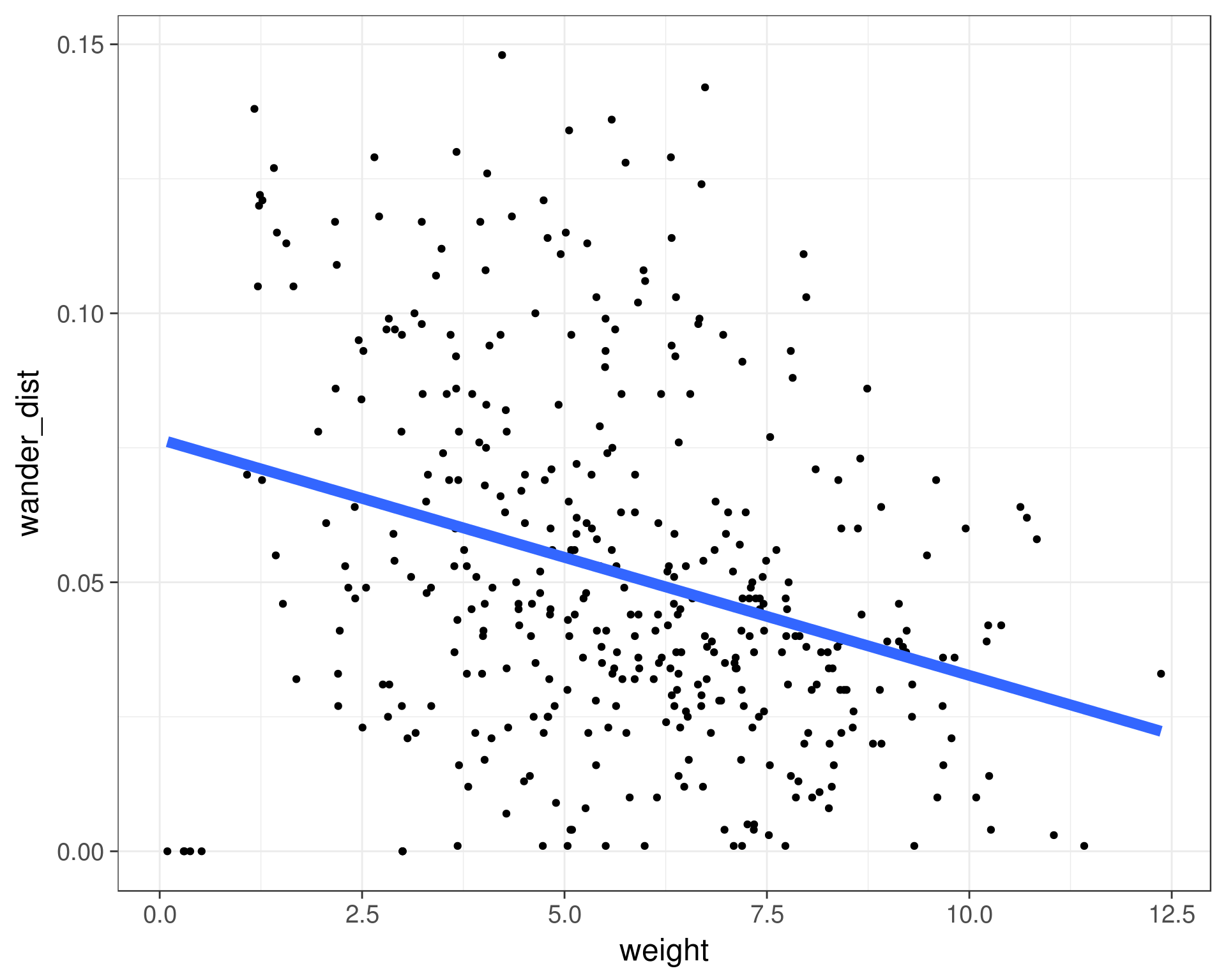
Simple linear regression estimates the linear relationship between two variables, an outcome variable y, and an explanatory variable x.

To fit a linear regression in R, we can use the lm() function (think linear model). We use the formula notation, y~x where y is the name of your outcome variable, and x is the name of your explanatory variable, both are unquoted. The easiest way to view the results interactively is with the summary() function.

weight_fit <- lm(formula = wander_dist ~ weight, data = cats)
summary(weight_fit)

---

In this case, the summary function returns an object that provides a lot of interesting information when printed out. It also stores that information as part of the object, things like the terms used in the model, the coefficients of the model estimates, and the residuals of the model. This is nice if we want to do something programmatic with the results.

---

9.0.2 Multiple Linear Regression

We aren’t restricted to just one explanatory variable in linear regression. We can test the effect of a linear relationship between multiple explanatory variables simultaneously. In the lm function, we just add extra variable names in the formula separated by +’s.

wander_fit <- lm(formula = wander_dist ~ weight + age , data = cats)
summary(wander_fit)

---

9.0.2 Challenge

Fit a model predicting wander_dist and include weight, age, and fixed as predictors. What is the estimate for the effect of being fixed on the wandering distance?

wander_fit <- lm(formula = wander_dist ~ weight + age + fixed, data = cats)
summary(wander_fit)

---

If an explanatory variable is not binary (coded as 0s or 1s), we can still include it in the model. The lm function understands factors to be categorical variables automatically and will output the estimates with a reference category.

wander_fit <- lm(formula = wander_dist ~ weight + age + factor(coat) + sex, data = cats)
summary_fit <- summary(wander_fit)
summary_fit['coefficients']

9.0.2 Challenge

What command will return the r-squared value from the summary_lm_fit object after running these commands:

wander_fit <- lm(formula = wander_dist ~ weight + age + fixed, data = cats) summary_lm_fit <- summary(wander_fit)

---

The lm function also can estimate interactions between explanatory variables. This is useful if we think that the linear relationship between our outcome y and a variable x1 is different depending on the variable x2. This can be accomplished by connecting two variables in the formula with a * instead of a +.

9.0.2 Challenge

Fit a linear regression model estimating the relationship between the outcome, wandering distance (wander_dist) and explanatory variables age (age), weight (weight), with an interaction between age and weight. What is the coefficient associated with the interaction between age and weight?

wander_fit <- lm(formula = wander_dist ~ weight * age, data = cats)
summary(wander_fit)